Circular Buffer

Circular Buffer or Ring Buffer is an interesting data structure, that I honestly didn't have the chance or the need to use before. Until, I decided to connect to LMAX and start getting their feed in real time. It's a quite known problem in computer science literature, the thing that you learn in your first algorithm course, The Producer-Consumer problem. Using a semaphore or a blocking queue or concurrent queue.. will do the trick, but I wanted to have a fast producer and a fast consumer without blocking, controlling the memory size and reducing CPU usage.
Here I am searching the web, searching in my library if I missed any interesting data structure for my case, even s The Algorithm Design Manual  by Steven S. Skiena that I consider a must have, didn't find the answer. After sometimes a friend of mine told me about a presentation How to do 100k TPS less than 1ms Latency my surprise was is that the same people that I want to connect to their system already solved this problem. Great presentation, Martin Thompson talks about "Mechanical Harmony" and how they did achieve it in LMAX, one of the interesting point that I tried later for my case was the single, fixed-sized buffer.  Looking at few implementation online, from the C++ wikipedia exemple to one academic implementation of Neal R. Wagner.
After few Unit test where I varied Producer-Consumer speed, I found that sometimes the consumer read empty values where it shouldn't. Looking again the dequeue method

public T dequeue() {
  if (!isEmpty()) {
   readCount++;
   size--;
   head = (head + 1) % maxSize;
   T result = queue[head];
   queue[head] = null;
   return result;
  } else {
   return null;
  }
 }

There is a chance that we read the head before writing it even if we did pass the condition that the queue is not empty. Therefore I added king of double check, but without the locking, see below.

import java.util.concurrent.atomic.AtomicInteger;

public class CircularBuffer {
 private final int maxSize;
 private volatile int head = 0;
 private volatile int readCount = 0;
 private volatile int writeCount = 0;
 private volatile int tail = 0;
 private final AtomicInteger size = new AtomicInteger(0);
 private final T[] queue;

 @SuppressWarnings("unchecked")
 public CircularBuffer(int size) {
  this.maxSize = size;
  this.queue = (T[]) new Object[this.maxSize];
 }

 public int getReadCount() {
  return readCount;
 }

 public int getWriteCount() {
  return writeCount;
 }

 public int getSize() {
  return size.get();
 }

 public T dequeue() {
  if (!isEmpty()) {
   int tmp = (head + 1) % maxSize;
   T result = queue[tmp];
   if (result == null) {
    return null;
   }
   readCount++;
   size.decrementAndGet();
   head = tmp;
   queue[head] = null;
   return result;
  } else {
   return null;
  }
 }

 @Override
 public String toString() {
  return "Write #" + writeCount + " Read #" + readCount + " Size #" + size.toString();
 }

 public void enqueue(T element) {
  if (!isFull()) {
   writeCount++;
   size.incrementAndGet();
   tail = (tail + 1) % maxSize;
   queue[tail] = element;
  } else {
   throw new RuntimeException(" Circular Buffer is Full");
  }
 }

 public boolean isEmpty() {
  return size.get() == 0;
 }

 public boolean isFull() {
  return maxSize == size.get();
 }

 public synchronized String printStatus(javascript:void(0)) {
  StringBuffer sb = new StringBuffer();
  for (int i = 0; i < maxSize; i++) {
   if (queue[i] != null)
    sb.append("\nqueue[" + i + "]=" + queue[i]);
  }
  return sb.toString();
 }
}

Option pricing using finite difference method - Matlab

During the course Quantitative & Computational Finance within the maths department at UCL. We were asked to price 4 types of option, European call option, European Put option, and Binary options using the finite difference method. This post describe the the Black-Scholes equation and its boundary conditions, the finite difference method and finally the code and and the order of accuracy.
For the matlab code in this post I used the java brush, therefore the comments will need to be changed from // to %. I know you would ask, why I didn't use a Matlab brush in the first place, well I am using the SyntaxHighlighter and looking at this comment "Note from author: the long list of functions (1300) can make the browser unresponsive when you use this brush."put me off.

I Black-Scholes equation

The black-Scholes equation \[\frac{\delta V}{\delta t}+\frac{1}{2}\sigma^2 S^2 \frac{\delta^2 V}{\delta S^2}+r S \frac{\delta V}{\delta S} - r V = 0 \]

Where $S=\mbox{Stock price},\sigma=Volatility,r=\mbox{Interest Rate},V=\mbox{Option Value}$
This is a linear parabolic equation partial differential equation.
In terms of Greeks, the Black-Scholes equation can be written as follow \[ \Theta = -\frac{1}{2} \sigma^2 S^2 \Gamma - r S \Delta + r V\]
Final & Boundary Conidions

1. Final condition is the Payoff 
2. Boundary conditions at $S=0\$ and at $S=\infty\$

European Call Option

1. Payoff $C_{E}(S,T) = max(S-E,0)\$
2. Boundary Conditions : 
1. At $S=0 \qquad V(S,T) = 0\$
2. At $S=\infty \qquad V(S,T) = S\$

Black-Scholes closed from solution

The closed form solution for the Black-Scholes equation for a European Call option is

\[C(S,T) = S\quad N(d_1) - E\quad e^{-r(T-t)}\quad N(d_2)\]

where \[d_1 = \frac{log(\frac{S}{E}) + (r+\frac{1}{2}\sigma^2)(T-t)}{ \sigma \sqrt{T-t}}\],

\[d_2 = \frac{log(\frac{S}{E}) + (r-\frac{1}{2}\sigma^2)(T-t)}{ \sigma \sqrt{T-t}}\]

and $N\$ is the cumulative distribution function of a standard normal.

Using the Call-Put parity equation $CALL-PUT = S - e^{-r (T-t)} N(-d_2)\$ we can also rite the put formula  \[P(S,T) = -S\quad N(-d_1) + E\quad e^{-r(T-t)}\quad N(-d_2)\]

For Binary type options, also called cash-or-nothing the Call and Put values:

\[C_B(S,T) =e^{-r(T-t)}\quad N(d_2)\]

 \[P_B(S,T)=e^{-r(T-t)}\quad (1-N(d_2))\]

II Finite Difference Method 

Finite difference method is a numerical methods for approximating the solutions to differential equations using finite difference equation to approximate derivative.

The finite-difference grid usually has equal time step, the time between nodes is equal S steps.

The time step is $\delta t\$ and the asset step is $\delta S\$. Thus the grid is made up of points at asset Values  $S=i\delta S\$ and times $t= T-k \delta t\$ where $0\leq i\leq l \$ and $0\leq k\leq K \$.

$ I \delta S\$ is our approximation of infinity, in this exercise we will use $S_\infty = 2 \cdot Strike\$

Thus we can write the option value at each of these grid point as \[V^{k}_{i}=V(i\delta S, T-k\delta t)\]

So that the superscript is the time variable and the subscript is the asset variable.

Now we will use the Black-Scholes Greeks notation to approximate theta, gamma and delta

Approximating $\Theta\$

The definition of the first derivative of V is \[\frac{\delta V}{\delta t} = \lim\limits_{\delta t \to 0} \frac{V(S,t+\delta t) - V(S,t)}{\delta t} \]

It follows that we can approximate the time derivative from our grid of values using the backward difference of time: \[\frac{\delta V}{\delta t}(S,t) \approx \frac{V^{k}_{i}-V^{k+1}_{i}}{\delta t} + O(\delta t) \]

This is the approximation of the option's theta. It uses the option value at two points of the grid V(k,i) and V(k+1,i). This approximation is one order accurate in delta t and we will see later  that later in the examples.

Approximating $\Delta\$

The same idea can be used to approximate the first order in S derivative, the delta. From a Taylor series expansion of the option value about the point $S+\delta S,t\$ we have \[V(S+\delta S,t)=V(S,t) + \delta S \frac{\delta V}{\delta S}(S,t) + \frac{1}{2}\delta S^2 \frac{\delta^2 V}{\delta S^2}(S,t)+O(\delta S^3)\]

Similarly,  \[V(S-\delta S,t)=V(S,t) - \delta S \frac{\delta V}{\delta S}(S,t) + \frac{1}{2}\delta S^2 \frac{\delta^2 V}{\delta S^2}(S,t)-O(\delta S^3)\] Subtracting from the other, dividing by $ 2\delta S\$ and rearranging gives \[\frac{\delta V}{\delta S}(S,t) = \frac{V^{k}_{i+1}-V^{k}_{i-1}}{2\delta S}+O(\delta S^2)\]  

Approximating $\Gamma\$

The gamma of an option is the second derivative of the option with respect to the underlying, The natural approximation is \[\frac{\delta^2 V}{\delta S^2}\approx \frac{V^{k}_{i+1}-2V^{k}_{1}+V^{k}_{i-1}}{\delta S^2} + O(\delta S^2)\] This approximation is also a second order accurate in $\delta S\$ as the approximation the $\Delta\$ and will show this also later.

The Explicit Finite-Diffrence Method

Calculation of the Greeks using the backward difference

Now we plug our previous Greeks approximation into the Black-Scholes equation \[\frac{V^{k}_{i}-V^{k-1}_{i}}{\delta t}+\frac{1}{2}\sigma^2(i^2\delta S^2) [\frac{V^{k}_{i-1}-2V^{k}_{i}+V^{k}_{i+1}}{\delta S^2}] +r i\delta S [\frac{V^{k}_{i+1}-V^{k}_{i-1}}{2\delta S}]- r V^{k}_{i}=0\] Rearranging \[V^{k-1}_{i}= \alpha_{i} V^{k}_{i-1} + \beta_{i} V^{k}_{i} + \gamma_{i} V^{k}_{i+1}\] with \[\alpha_{i} = \frac{1}{2}\sigma^2 i^2 \delta t - \frac{1}{2} i r \delta t\] \[\beta_{i}= 1 - \sigma^2 i^2 \delta t - r \delta t\] \[\gamma_{i}=\frac{1}{2}\sigma^2 i^2 \delta t + \frac{1}{2} i r \delta t\]
The finite difference equation is valid everywhere inside the grid that is not valid on the boundaries. Therefore we need to define the boundaries depending on the option type we are valuing.

Final & Boundary conditions

For a European Call opation at t = T(expiry); i = I \[Payoff V(S,t) = max(S-E,0)\] Thus \[V^{k}_{i} = max(i \delta S-E, 0) \] where $ 0\leq i \leq l \$

At S = 0 

The Black-Scholes equation become \[\frac{\delta V}{\delta t}=r V \to V^{k}_{i}-V^{k-1}_{i}=r V^{k}_{i}\delta t\] But at $S=0,i =0,V^{k}_{0}-V^{k-1}_{0}=rV^{k}_{0}\delta t\$ Thus $V^{k-1}_{0}=(1-r\delta t)V^{k}_{0}\$

At $t=\infty\$

The probability of S falling under E becomes negligible, also small changes in S fo not affecto the option price, then $\Gamma=\frac{\delta \Delta}{\delta S}=0\$ (For European Call option) \[\Gamma\approx\frac{V^{k}_{i-1}-2V^{k}_{i}+V^{k}_{i+1}}{\delta S^2}=0\] 

At i = I

This is the upper boundary condition \[V^{k-1}_{i}=(\alpha_{I}-\gamma_{I})V^{k}_{I-1}+(\beta_{I}+2\gamma_{I})V^{k}_{I})\] Finally for the stability criteria we will choose $\delta t \leq \frac{1}{I\sigma^2}\$.

III Code and Results

Here is the matlab implementation of the finite difference method. We used the same fixed parameters i.e volatility =0.2, Interest Rate =0.05, Strike Price = 100, current price is the discounted value of the strike price $S=100 e^{-rT}/$.

For each type of option we vary the time step and the asset price to show that the method is first order and second order accurate in $\delta t\$ and $\delta S\$ in turn. 

We also defnie the $\alpha,\beta and \gamma\$ externally for clarity.

The $\alpha\$ function code

function [ alpha ] = alphaN( n, sigma, r,dt )
  //ALPHAN return the alhpa value 
  //for Finite Difference Method
  //From the Black-Sholes FDM equation
  //Alpha =0.5*(sigma^2)*(n^2)*dt-0.5*n*r*dt;
     alpha = 0.5 * (sigma^2) * (n^2) * dt - 0.5 * n * r * dt;
end

The $\beta\$ function code

function [ beta ] = betaN( n, sigma, r,dt )
//BETAN return the beta value for Finite Difference Method
//From the Black-Sholes FDM equation
//betaN = beta = 1 - (sigma^2) * (n^2) * dt - r * dt;
 
beta = 1 - (sigma^2) * (n^2) * dt - r * dt;
 
end

The $\Gamma\$ function code

function [ gamma ] = gammaN( n, sigma, r,dt )
//GAMMAN return the gamma value for Finite Difference Method
//From the Black-Sholes FDM equation
//gamma = 0.5 * (sigma^2) * (n^2) * dt + 0.5 * n * r  * dt;
 
gamma = 0.5 * (sigma^2) * (n^2) * dt + 0.5 * n * r  * dt;
 
end

We have also defnied the results for the closed form solution for a European Call and put option and similarly for the binary options.

Closed form solution for European Call option

function [ val ] = BS_CALL( S, E , r , sigma ,T , t )
//BS_CALL Closed form solution using the Black-Scholes 
//equation to price a european CALL option
 
d1 = (log( S/E) + ( r + 0.5 * sigma^2) * (T-t))/(sigma * sqrt(T-t));
 
d2 =  d1-sqrt(T-t)*sigma;
 
val = S * normcdf(d1) - E* exp(-r *(T-t)) * normcdf(d2);
 
end

Closed form solution for European Put option

function [ val ] = BS_PUT( S, E , r , sigma ,T , t )
//BS_PUT Closed form solution using the Black-Scholes 
//equation to price a european PUT option
d1 = (log( S/E) + ( r + 0.5 * sigma^2) * (T-t))/(sigma * sqrt(T-t));
 
d2 =  d1-sqrt(T-t)*sigma;
 
val = -S * normcdf( - d1) + E * exp( -r * (T-t) ) * normcdf( - d2 );
 
end

Closed form solution for a European Call option (Cash-or-nothing)

function [ val ] = BS_CALL_B( S, E , r , sigma ,T , t )
//BS_CALL_B Closed form solution using the Black-Scholes 
//equation to price a european CALL option for a Cash or nothing option
 
d1 = (log( S/E) + ( r + 0.5 * sigma^2) * (T-t))/(sigma * sqrt(T-t));
 
d2 =  d1-sqrt(T-t)*sigma;
 
val = exp( -r * (T-t) ) * normcdf(d2);
 
end

Closed form solution for a European Put option (Cash-or-nothing)

function [ val ] = BS_PUT_B( S, E , r , sigma ,T , t )
//BS_PUT_B Closed form solution using the Black-Scholes 
//equation to price a european CALL option for a Cash or nothing option
 
d1 = (log( S/E) + ( r + 0.5 * sigma^2) * (T-t))/(sigma * sqrt(T-t));
 
d2 =  d1-sqrt(T-t)*sigma;
 
val = exp( -r * (T-t) ) * (1- normcdf(d2));
 
end

Here we define the option value function for a European Call and put option with respective payoff condition max(S-E,0) and mad(E-S,0). we notice that the code is similar only the payoff function can be reversed depending on the option type i.e call or a put.

Option Value Function

function [ Err_perc dt ds ] = Option_Value( S,vol, Int_Rate, PType, Strike, Expiration, NAS )
//OPTION_VALUE 
// vol : volatility
// Int_Rate : Interest Rate
// Option Type:  Put/Call
// Strike : Strike price
// Expiration : Experiy date
// NAS : number os asset steps
ds = 2 * Strike / NAS; //Infinity is defined as twise the strike price
dt = 0.9 / (vol^2 * NAS^2) ;//For stability 
NTS = round( Expiration / dt ) + 1; //Number of time steps
dt = Expiration / NTS; // to ensure the expiration is an integer number of time steps
v = zeros(NAS, NTS); //option price grid
q = 1;
if ( strcmp(PType , 'PUT'))
    q = -1 ;
end 
//Define boundary condition at expiriy
temp = (0:NAS-1);
V( :,NTS) = max( q * ( temp * ds - Strike) , 0);
%at S = 0;
%V(m-1, 0) = (1 - r dt) * V(m,0)
for i = NTS : -1 : 2
    V(1,i-1) = ( 1 - Int_Rate * dt) * V(1, i); 
end
for j = NTS : -1: 2
    for i =  2: NAS -1
        V(i,j-1) = alphaN(i,vol,Int_Rate,dt) * V(i-1,j) + 
                            betaN(i,vol,Int_Rate,dt) * V(i,j) +
                                gammaN(i,vol,Int_Rate,dt) * V(i+1,j);
    end
    //Satisfy boundary conditions
    V(NAS,j-1) = (alphaN(i,vol,Int_Rate,dt) -  
                                gammaN(i,vol,Int_Rate,dt) ) * V(NAS-1,j) +
                                    ( betaN(i,vol,Int_Rate,dt) + 
                                            2*  gammaN(i,vol,Int_Rate,dt) ) * V(NAS,j);
end
cFormSolution = 0;
if ( strcmp(PType , 'CALL'))
    cFormSolution = BS_CALL( S, Strike , Int_Rate , vol ,Expiration , 0)
else
    cFormSolution = BS_PUT( S, Strike , Int_Rate , vol ,Expiration , 0)
end 
//pick up the option price at t = 0
index = round((S/ds)+1)
//Error with the closed form solution
Err = cFormSolution - V(index,1);
//Error with the closed form solution in percentage
Err_perc = abs( Err/cFormSolution )
end

Binary option value function

function [ Err_perc dt ds ] = Option_Value_B( S,vol, Int_Rate, PType, Strike, Expiration, NAS )
//OPTION_VALUE 
// vol : volatility
// Int_Rate : Interest Rate
// Option Type:  Put/Call
// Strike : Strike price
// Expiration : Experiy date
// NAS : number os asset steps
ds = 2 * Strike / NAS; //Infinity is defined as twise the strike price
dt = 0.9 / (vol^2 * NAS^2) ;%For stability 
NTS = round( Expiration / dt ) + 1 //Number of time steps
dt = Expiration / NTS; // to ensure the expiration is an integer number of time steps
v = zeros(NAS, NTS);
q = 1;
if ( strcmp(PType , 'PUT'))
    q = -1 ;
end 
for i = 1 : NAS
    if( max( q * ( i * ds - Strike) , 0) >= 0 )
        V(i,NTS) = 1;
    else
        V(i,NTS) = 0;
    end
end
//at S = 0;
//V(m-1, 0) = (1 - r dt) * V(m,0)
for i = NTS : -1 : 2
    V(1,i-1) = ( 1 - Int_Rate * dt) * V(1, i); 
end
for j = NTS : -1: 2
    for i =  2: NAS -1
        V(i,j-1) = alphaN(i,vol,Int_Rate,dt) * V(i-1,j) + betaN(i,vol,Int_Rate,dt) * V(i,j) + gammaN(i,vol,Int_Rate,dt) * V(i+1,j);
    end
    %Satisfy boundary conditions
    V(NAS,j-1) = (alphaN(i,vol,Int_Rate,dt) -  gammaN(i,vol,Int_Rate,dt) ) * V(NAS-1,j) + ( betaN(i,vol,Int_Rate,dt) + 2*  gammaN(i,vol,Int_Rate,dt) ) * V(NAS,j);
end
cFormSolution = 0;
if ( strcmp(PType , 'CALL'))
    cFormSolution = BS_CALL_B( S, Strike , Int_Rate , vol ,Expiration , 0)
else
    cFormSolution = BS_PUT_B( S, Strike , Int_Rate , vol ,Expiration , 0)
end 
index = round((S/ds)+1)
Err = cFormSolution - V(index,1);
Err_perc = abs( Err/cFormSolution )
end

In the figure below we output the call option values by the explicit finite-difference method.

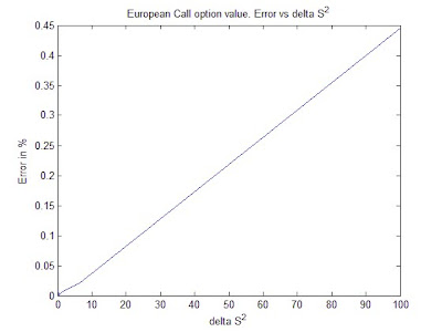
In the following we will show that the finite-difference methods is first order and second order accurate in $\delta t\$ and $\delta S\$ in turn by plotting the Error against $\delta t\$ and $\delta S^2\$ in both plot we expect to have a linear plot.

European Call option values Error Vs. $\delta t\$

European Call option values Error Vs. $\delta S^2\$

European Put option values Error Vs. $\delta t\$

European Put Option values error Vs. $\delta S^2\$

Plotting the error in percentage against the $\delta t\$ and $\delta S^2\$ for the European call and put option for both payoff function continuous and binary, we clearly see that the error is linear in $\delta t\$ and $\delta S^2\$.

The smaller the steps are in $\delta t\$ and $\delta S^2\$ the precise the finite-difference method is but this come with an expensive computation time.

References

Paul Wilmott Introduces Quantitative Finance, Second Edition, by Paul P.Wilmott

Options, Futures, and Other Derivatives (Prentice Hall Series in Finance), Seventh Edition, by John C.Hull